The past decade has seen a rise in the application of machine learning to all walks of life – from low impact applications like music recommendation systems to high-stakes uses, namely healthcare and autonomous vehicles. In the case of the former, the odd erroneous prediction has minimal negative consequences. What is the worst that can happen – a connoisseur of the opera is recommended the latest Justin Bieber song? However, in the latter case, it is very important that the models make the right prediction, or at the very least, inform the user that they do not know the answer for a given input. Unfortunately, most of the neural network models in production are extremely overconfident when they make a prediction, even when it is the wrong answer.
Reports suggest that the influence of AI in these crucial fields is only going to increase in the coming years. Therefore, it is imperative that the limitations of these systems are made common knowledge, and that potential solutions are explored. This blog post aims to do exactly that.
At Pex, the motivation to incorporate uncertainty estimation stemmed from observing a lot of out-of-distribution data while building an automatic video categorizer for user-generated content (UGC). What does this mean? To put it simply, the video categorizer was trained to classify a video into one of a few classes, such as sports, health and fitness, standup comedy etc. However, we observed that a significant chunk of the UGC did not belong to any of the classes we were interested in. They were either abstract one off classes, or a class we were not interested in predicting. Given these circumstances and Pex’s strong emphasis on precision, a deeper dive into uncertainty modeling was necessary.
Types of uncertainty
Before introducing some of the solutions, it is necessary to understand the types of uncertainty. There are two types of uncertainty – aleatoric uncertainty and epistemic uncertainty. Epistemic uncertainty is the uncertainty in the parameters of a model. The easiest way to reduce epistemic uncertainty is by gathering more data. In an ideal world with infinite data and infinite model size, there is zero epistemic uncertainty. Aleatoric uncertainty on the other hand refers to uncertainty in the observed data – this is usually some kind of noise or perturbation of the input signal. This uncertainty cannot be reduced by training the model with more data.
Solutions in the literature
Historically, Gaussian processes have been the gold standard for uncertainty modeling. However, they do not scale well with larger data and lack the computational complexity of modern neural networks. The past few years have seen efforts to model uncertainty within the neural networks framework. There are techniques that have seen relative success, with minor additions to model architecture/training/inference that should be easy to implement.
One such approach is MC dropout. In this method, dropout is applied at both training and test time. At test time, the data is passed through the network multiple times, with different parameters being dropped at each run. In the end, the outputs are averaged over the number of runs to output the probability, P(Y|X)
Another popular approach is Deep ensembles. A neural network is trained from scratch, multiple times on the same dataset. At test time, the data is passed through all these models, and the final output is the average of the combined outputs. The obvious drawback is that this leads to an increase in storage. However, training the networks from scratch allows the networks to find minima in the loss landscape that are well separated.
A technique that promises to improve calibration is Temperature scaling. In this method, the logits in the output layer are divided by a learned parameter called temperature. This calibration is tuned on the validation set. In the experiments, the authors observed that the calibration works well for in distribution test data, however the same cannot be extended to out of distribution datasets
Bayesian neural network
In our experiments with the video categorizer, we had the most success with a Bayesian neural network. A successful model for us was the one with the lowest false positive rate.

The above is the general form of an equation to perform inference on an input X, to obtain the probability distribution of the output Y, given model parameters w, and the training dataset D. Ideally, an integral would be computed over all possible model parameters, weighted by their probability. This is known as marginalization over parameters w. Unfortunately, this operation is not tractable because the parameter space of w is so large that it is not feasible to integrate over it.
Most of the models in production today perform inference using only one setting for the model parameters w. These parameters are learned by maximum likelihood estimation. This can result in overconfident wrong answers when the model makes errors, leading to poor uncertainty estimation.
So, it is important to learn a distribution for the model weights. There are two ways to do this – MCMC algorithms or Variational Bayes. MCMC is a reliable method, but it can be very slow to converge and does not scale to large datasets. In the next section, we explore Variational Bayes. This is less accurate than MCMC but more scalable.
Posterior approximation with Variational Bayes
Given that the true distribution of the posterior p(w | D) is intractable, one solution is to approximate it with a simpler distribution. This is known as Variational Bayes, where a distribution parameterized by ? is used as a proxy for the true distribution. This distribution is learnt by minimizing the KL divergence between the parameterized distribution q(w | ?) and the posterior p(w | D). Mathematically, we write it as

What is the KL divergence?
This is a distance measure defined to understand how close two probability distributions are to each other. An important property of the KL divergence is that it is not symmetric. Given two probability distributions, p and q, KL divergence is defined as,

A lower value of KL divergence means that the distribution q is close to p. When q = p, the KL divergence is 0.
The gif below illustrates why the KL divergence is not symmetric, and why it is important to know that. While calculating KL(q || p), the only portion of the input space that contributes to the integral is where q(x) has high probability mass. So, for the KL divergence between q and p to be low, it is sufficient for p to have non zero probability mass in that region. In the illustration, q can serve as a good proxy for p. However, the opposite is not true. When we compute KL(p || q), the distribution q has close to 0 probability mass around the second mode of p. As a result, the term p(x)q(x) will tend to reach infinity. Due to this large value for KL divergence, p cannot serve as a proxy for q.

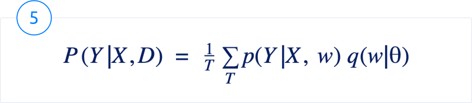
So, after finding the parameters (details on the optimization process can be found in this paper) that minimize the function KL(q(w | ?) || p(w | D)), we can rewrite eq (1) as

It is easier to sample weights from this distribution. However, it is still impossible to traverse the entire space of w to compute the integral. So, we run inference T times – where T is a hyperparameter, and average over all the outputs to get the final prediction.
The larger the value of T is, the better the uncertainty estimation. This however comes with the cost of larger inference time. Another drawback of this method is that it can approximate only one mode of the true probability distribution.
Evaluation
There are two important evaluations that need to be performed, along with calculating the accuracy on the test set – calibration error, and performance on out of distribution data.
The calibration error gives us an indication of how close a model’s output confidence is related to the true probability. For example, if we have 100 data points, all whose model outputs are at a confidence of 80%, we should expect that 80 of those predictions are accurate and the rest are wrong. If the number of accurate predictions are more than 80, we say that the model is under confident. If it is less than 80, we say the model is overconfident.
To test how the model performs on out of distribution data, we feed the model out of distribution data. In the example below, a model trained on MNIST is forced to make predictions on images from CIFAR-10. For those unfamiliar with the two datasets, MNIST is a dataset of handwritten digits ranging from 0 to 9, and CIFAR 10 is a dataset of 10 different object classes, viz: cats, dogs, airplanes etc. What this means is, a model which only knows about numbers should not make confident predictions about image classes such as cats and dogs.


The above two plots show the histogram of confidence scores of a regular neural network and a Bayesian neural network of similar architecture. We see that the bulk of the predictions of the regular neural network have over 90% confidence. On the other hand, hardly any of the Bayesian neural networks predictions exceed 90%. In fact, the bulk of the predictions are below 50% confidence.
Conclusion
Uncertainty modeling is an exciting area of study, and a lot of research groups are involved in improving upon existing methods. As AI applications continue to increase their influence on modern society, it is important to make sure we know that the models know when they don’t know.
Want to work on similar exciting problems with us? Check out our open positions.