There are many exciting problems that can be solved by training machine learning models on large, audio datasets – distinguishing speakers, identifying instruments in music, and translating speech from one language to another to name a few.
The question is, how can we train a machine learning model to do inference on audio data? The answer requires picking out signals from the data that represent what humans perceive as musically or linguistically important.
In this blog post, we will briefly describe what sound is, how it is represented digitally, and how we interpret sound. We will then demonstrate how to extract relevant features from sound in Python using packages like NumPy and Essentia.
Sound and Sound Waves
A sound wave is a pressure wave caused by an object vibrating in a medium, like air. These waves can be described by how fast they vibrate (frequency) and the magnitude of their vibrations (amplitude). When sound waves hit our ears, they stimulate microscopic hair cells that send nerve impulses to our brains. These impulses are what we perceive as sound. We interpret the frequency of sound waves as pitch and the amplitude as volume.
We typically hear frequencies between 20 and 20,000 Hz (vibrations per second), with higher frequencies corresponding to higher pitches. It is important to note, however, that we have a harder time distinguishing between higher pitches than lower ones. Similarly, we perceive sound waves with larger amplitudes as louder and have a harder time distinguishing between louder sounds. As a consequence, we will engineer our features to account for this.
Digital Audio Signals
It is important to spend a minute discussing how audio signals are stored digitally. When we record sound, we are periodically measuring the amplitude of a sound wave in time. These measurements are called samples and typically comprise the bulk of the data contained in audio files. The data may consist of multiple streams of audio samples, known as channels, that measure diff – think about the different sounds coming out of the left and right speakers of stereo systems, for example.
When we record audio, we must decide how often to take measurements. This is called the sampling rate, or number of samples recorded per second. This value is also contained in the audio file in lieu of time and determines the highest frequency we can detect in the signal, or the Nyquist frequency.
There are many audio file formats that exist, but for the rest of this blog post we will run analysis on uncompressed data in a wav file. We can use SoX to determine the sample rate and number of channels in this example file.
soxi example.wav

Input File     : 'example.wav'
Channels       : 2
Sample Rate    : 44100
...
To load and analyze the data, we will use Essentia. We see above that example.wav has two channels, which we down-mix into one using Essentia’s MonoLoader. The data are in the form of a numpy array, where the columns correspond to the number of channels (in this case one). Let us extract the first second, or first 44100 samples, of audio.
| # Extract the first second of audio | |
| import essentia | |
| import essentia.standard | |
| loader = essentia.standard.MonoLoader(filename='example.wav', sampleRate=44100) | |
| audio = loader() | |
| sec_audio = audio[0:44100] |
We can then plot the waveform using Matplotlib and Seaborn.
| # Plot the first second of audio | |
| import matplotlib | |
| import matplotlib.pyplot as plt | |
| import seaborn as sns | |
| plt.plot(sec_audio) | |
| plt.title('Sound Wave') | |
| plt.xlabel('Samples') | |
| plt.ylabel('Amplitude') |

Representing Pitch and Volume
So how do we transform the audio data into linguistically important features that capture pitch and volume? Since we can represent any wave as a sum of sine and cosine functions with different frequencies and amplitudes, we will describe the original wave in terms of these components. This is done by performing a Fast Fourier Transform, or FFT, to produce a spectrum of frequencies.
However, when performing a Fourier transform, one assumes that the audio signal is stationary or remains constant in time. This assumption does not hold true for most audio files we are interested in. We therefore perform multiple FFTs on short segments of our waveform that are approximately stationary, which we refer to as frames. However, the lowest frequency we can resolve is equal to the inverse of the frame length, so we do not want to make the frames too small. A typical choice for this length is 25 ms, which means that 40 Hz is the lowest frequency we can detect.
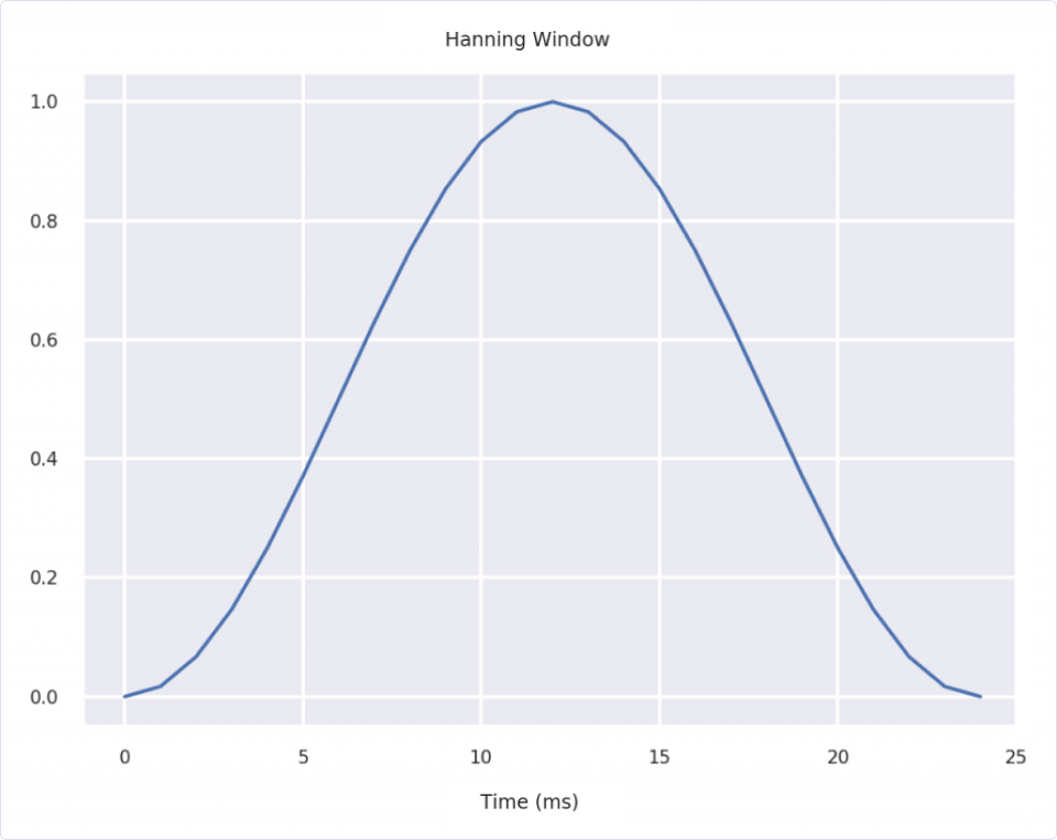
Furthermore, we apply a window function over each frame to minimize spectral leakage. A popular choice is the Hanning window, plotted using numpy and matplotlib below. Since we lose information near the edges of the window where the function goes to zero, we perform FFTs on overlapping windows, typically shifted by 10 ms.
| import numpy as np | |
| window = np.hanning(25) | |
| plt.plot(window) | |
| plt.title('Hanning Window') | |
| plt.xlabel('Time (ms)') |
In Essentia, we can compute the power spectrum, or the power of each frequency component, as follows:
| from essentia.standard import Windowing, PowerSpectrum | |
| # Compute the spectrum of a frame | |
| w = Windowing(type='hann') | |
| spectrum = PowerSpectrum(size=1024) | |
| frame = audio[0:1024] | |
| spec = spectrum(w(frame)) | |
| # Plot the spectrum of a frame | |
| plt.plot(spec) | |
| plt.title("Spectrum") | |
| plt.xlabel("Frequency (Hz)") | |
| plt.ylabel("Power") |
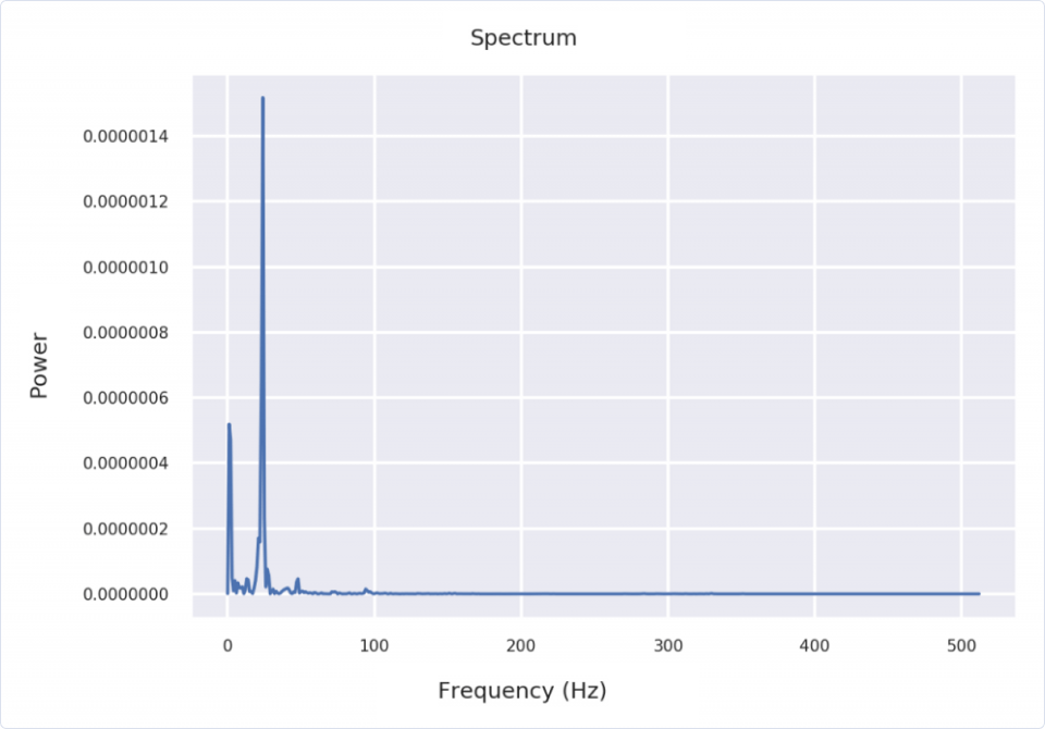
Careful readers may wonder why we are using 1024 samples per frame instead of 1103 (= 44100 Hz × 0.025 s). The answer is that the FFT algorithm works when the number of samples is a power of two (1024 = 2^10).
The next step is to determine which pitches are present in the frame. Remember how we said that humans are worse at distinguishing between high frequencies? Well, instead of having lots of high frequencies in our spectrogram that contribute practically nothing to our signal, it would be nice to represent these frequencies as a single pitch that contributes something more substantial. Consequently, we group similar sounding frequencies together and calculate their average power.
How do we know which frequencies are similar? Fortunately, scientists came up with a formula that maps frequency to equally spaced pitches, or mels.
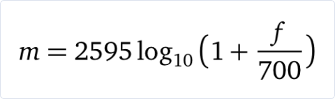
This formula is plotted below for the range of frequencies we are considering. As you can see, going from 5 kHz to 10 kHz corresponds to a larger jump on the mel scale than a jump from 15 kHz to 20 kHz.
| # Define function for computing mels | |
| def mel_formula(f): | |
| return 2595 * np.log(1 + f/700) | |
| # Frequency range | |
| f_low = 40 | |
| f_high = 44100 / 2 # Nyquist frequency | |
| f = np.linspace(f_low, f_high) | |
| # Plot relationship between frequency and mels | |
| plt.plot(f, mel_formula(f)) | |
| plt.title('Mel vs. Frequency') | |
| plt.xlabel('Frequency (Hz)') | |
| plt.ylabel('Mel Scale') |

To form the groups we divide our mel scale into equal segments called mel bands and call two frequencies similar if they belong to the same band. The optimal number of bands depends on your task and sampling rate. Popular choices for this number are 15 for 8 kHz audio, 23 for 16 kHz audio, and 25 or more for 44 kHz audio.
| # Compute the mel bands | |
| n_bands = 25 | |
| # The "+ 2" will make sense in a bit! | |
| m = np.linspace(mel_formula(f_low), mel_formula(f_high), n_bands + 2) | |
| print(m) |
[ 144.20376375  486.11200483  828.02024591 1169.92848699 1511.83672807
 1853.74496915 2195.65321023 2537.56145131 2879.46969239 3221.37793347
 3563.28617455 3905.19441563 4247.10265671 4589.01089779 4930.91913887
 5272.82737995 5614.73562103 5956.64386211 6298.55210319 6640.46034427
 6982.36858535 7324.27682643 7666.18506751 8008.09330859 8350.00154967
 8691.90979075 9033.81803183]
To get the frequencies of each mel band, we rearrange the formula above and convert back to hertz.

| def inverse_mel_formula(m): | |
| return 700 * (np.power(10, m/2595) - 1) | |
| # Convert back to frequency | |
| f = inverse_mel_formula(m) | |
| print(f) |
[9.55507531e+01 3.77517764e+02 7.59422328e+02 1.27668531e+03
1.97728178e+03 2.92619061e+03 4.21142116e+03 5.95217590e+03
8.30990625e+03 1.15032868e+04 1.58284972e+04 2.16866915e+04
2.96212054e+04 4.03679486e+04 5.49236595e+04 7.46383502e+04
1.01340518e+05 1.37506733e+05 1.86491338e+05 2.52837554e+05
3.42698856e+05 4.64409694e+05 6.29258498e+05 8.52534655e+05
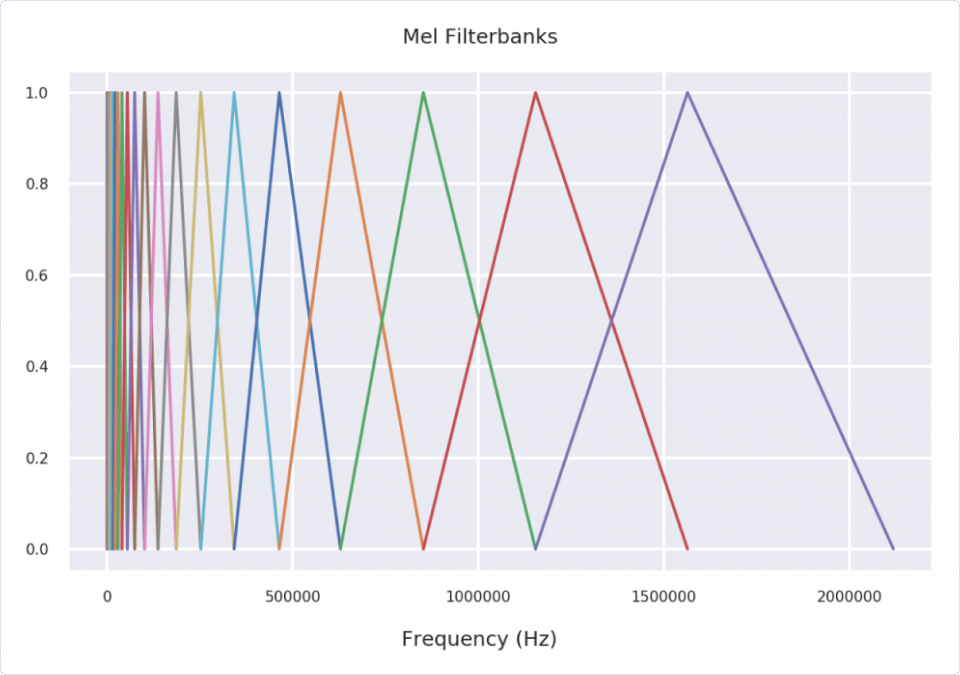
1.15494657e+06 1.56454232e+06 2.11931107e+06]We are now going to do something fancier than simply averaging the powers over each frequency group or bin. If we compute triangular, overlapping windows (that are centered over each bin) and multiply them by their corresponding powers, we can calculate moving, weighted averages.
Let’s go ahead and plot these windows, which are called mel filterbanks.
| for n in range(n_bands): | |
| plt.plot(f[n:n+3], [0, 1, 0]) # Does the "+ 2" make sense now? | |
| plt.title('Mel Filterbanks') | |
| plt.xlabel('Frequency (Hz)') |
Next, instead of doing the multiplication by hand, let’s use Essentia’s MelBands class to compute those weighted averages.
| from essentia.standard import MelBands | |
| # Compute the mel band powers | |
| melbands = MelBands(lowFrequencyBound=f_low, | |
| highFrequencyBound=f_high, | |
| inputSize=1024, | |
| numberBands=n_bands, | |
| type='magnitude', # We already computed the power. | |
| sampleRate=44100) | |
| mels = melbands(spec) | |
| # Plot the mel band powers | |
| plt.bar(np.arange(len(mels)), mels, align='center') | |
| plt.title('Mel Band Powers') | |
| plt.xlabel('Mel Bands') | |
| plt.ylabel('Power') |

Remember that humans are bad at distinguishing between loud and really loud noises too? Our perception of loudness is fairly subjective and depends on multiple factors, but it is related to the sound intensity level. The equation for relating the intensity of one sound to another is:

Where the unit of b is decibels and ? is the sound intensity, which is proportional to the power. I? is a standard reference value equal to 10^?12 watts per square meter, but in theory could be the intensity of any sound.
In our case, however, we should account for the relative loudness of each pitch by simply taking the logarithm of the mel powers. The reason being that although the power of a physical pressure wave is related to the power of its recorded signal, we can’t really apply the previous formula with its standard reference value to the recorded signal.
| from essentia.standard import UnaryOperator | |
| # Convert to decibels | |
| log10 = UnaryOperator(type='log10') | |
| log_mels = log10(mels) | |
| # Plot the mel band powers | |
| plt.bar(np.arange(len(log_mels)), log_mels, align='center') | |
| plt.title('Log of the Mel Band Powers') | |
| plt.xlabel('Mel Bands') | |
| plt.ylabel('Log of Power') |
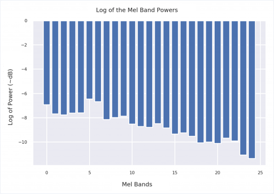
Furthermore, notice how taking the logarithm leveled the graph? Doing so also prevents us from losing important information in the next step.
Trimming the Fat
We can go ahead, perform all of these steps for every frame, and then chuck the results into a machine learning model. That being said, as the author of this StackExchange post explains, it is generally a good idea to de-correlate your data. By removing correlated data, you not only cut down on the size of your massive dataset, but you also make it possible for certain models to work.
We accomplish this task by performing a discrete cosine transform (DCT), which is similar to a discrete Fourier transform, on the log of the powers of the mel bands. The output of our DCT is a spectrum of the spectrum plotted above, called the mel-frequency cepstrum (the word “cepstrum” being a clever rearrangement of the letters in “spectrum”). You can think of the output as a description of the shape of the input, where the lower frequencies capture the majority of the spectrum’s topography. Since we compressed the input by taking the logarithm in the previous step, we can consider the first 12-20 cosine functions with the lowest frequencies and discard the rest without losing too much information.
We perform a DCT in Essentia using the appropriately named DCT class and plot the coefficients of the first 13 cosines.
| # Perform a DCT | |
| from essentia.standard import DCT | |
| dct = DCT(inputSize=n_bands, outputSize=13) | |
| mfccs = dct(log_mels) | |
| plt.bar(np.arange(len(mfccs)), mfccs, align='center') | |
| plt.title('Mel-Frequency Cepstrum') | |
| plt.xlabel('Cosines') | |
| plt.ylabel('Coefficients') |

These coefficients, called mel-frequency cepstral coefficients (MFCCs), are the final features used in many machine learning models trained on audio data!
Putting it all together
Instead of repeating the steps above for every frame in our audio file, we use Essentia’s MFCC class in addition to their FrameGenerator to easily compute MFCCs. As the documentation states, “there is no standard implementation” for computing MFCCs, and you may notice slight differences between the two methods.
| from essentia.standard import MFCC, FrameGenerator | |
| mfcc = MFCC(highFrequencyBound=f_high, | |
| lowFrequencyBound=f_low, | |
| inputSize=1024, | |
| numberBands=n_bands, | |
| numberCoefficients=13, | |
| type='magnitude', | |
| sampleRate=44100) | |
| # Compute MFCCs for all frames | |
| mfccs = [] | |
| for frame in FrameGenerator(audio, | |
| frameSize=1024, | |
| hopSize=512, | |
| startFromZero=True): | |
| _, coeffs = mfcc(spectrum(w(frame))) | |
| mfccs.append(coeffs) | |
| # Take the transpose so frames can be plotted on the x-axis | |
| mfccs = essentia.array(mfccs).T |
We can then plot our features.
| # Plot MFCCs | |
| plt.imshow(mfccs, | |
| aspect='auto', | |
| origin='lower', | |
| interpolation='none', | |
| cmap=plt.cm.Blues) | |
| plt.title("MFCCs") | |
| plt.xlabel("Frames") | |
| plt.ylabel("MFCCs") |
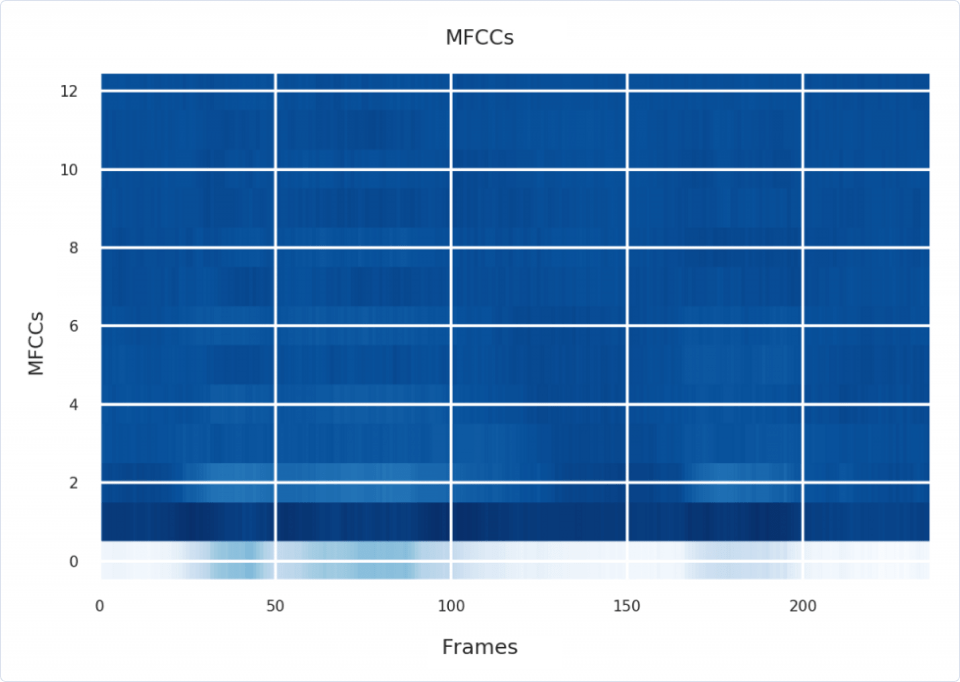
And there you have it?-?a nice set of audio features to train your machine learning model on. Since different instruments, speakers, and languages produce different types of sounds that can be characterized by changes in pitch and volume over time, we can uniquely describe each with sequences of MFCCs. Consequently, we can train a model to associate different MFCC signatures with different audio sources.
To summarize, here are the steps to compute MFCCs:
- Take Fourier transform of windowed frame.
- Map the frequency spectrum to the mel scale to account for human perception of pitch.
- Take logs of the powers of the mel spectrum to adjust for loudness and catch highly dynamic power values.
- Take the discrete cosine transform of the mel log powers to decorrelate the powers and drop part of the signal.
- Find the amplitudes or coefficients of the resulting spectrum, called MFCCs.
- Repeat for all frames, using overlapping windows.
Interested in working with machine learning models like this one?
Apply for a role at Pex! Check out our open positions.